In 1973, Wilcox published a paper presenting various indices of qualitative variation for social scientists. The problem is to find relevant statistical indices to measure the variation in nominal-scale (i.e. qualitative or categorical) data. Please see the Wilcox paper for more details on the rationale.

Wilcox presents six indices that can be used to measure qualitative variation. The qualvar package implements these indices so that R users can easily use them.

The indices

The DM (deviation from the mode)

According to Wilcox (1973, p. 327), ‘the measure can be thought of as an index of deviation from the modal frequency, analogous to the variance as a measure of deviation from the mean’. The formula for the DM is:

\[ 1 - \frac{\sum_{i = 1}^k (f_m - f_i)}{N(K-1)} \]

The ADA (average deviation analog)

According to Wilcox (1973, p. 328), the ADA is ‘an analog of the average or mean deviation’. The formula for the ADA is:

\[ 1 - \frac{\sum_{i=1}^k \left| f_i - \frac{N}{K}\right|}{2 \frac{N}{K}(K-1)} \]

The MDA (or MNDIF – mean difference analog)

According to Wilcox (1973, p. 328), the MDA is ‘an analog of the mean difference, a measure of variation that is discussed and used much less frequently than the average deviation or the standard deviation. It is defined as “the average of the differences of all the possible pairs of variate-values, taken regardless of sign”’. The formula for the MDA is:

\[ 1 - \frac{\sum_{i=1}^{k-1} \sum_{j=i+1}^k |f_i - f_j|}{N(K-1)} \]

The VA (variance analog)

According to Wilcox (1973, p. 329), the VA is ‘based on the variance, which is defined as the arithmetic mean of the squared differences of each value from the mean’. The formula for the VA is:

\[ 1 - \frac{\sum_{i=1}^k \left(f_i - \frac{N}{K}\right)^2}{\frac{N^2(K-1)}{K}} \]

The HREL index

According to Wilcox (1973, p. 329), and following Senders (1958), the HREL is ’a measure originally developed by engineers for use in specifying the properties of communications channels. The rationale for HREL is presented in terms of guessing by Virginia Senders (supplementing the mode as best guess): “What we need is a measure of uncertainty, or of ‘poorness of a guess,’ which will be high when the number of alternative possibilities is high, and low when some ofthe possibilities are much more likely than others. One possible measure is the average number of questions we have to ask to specify the correct alternative’. The formula for the HREL is:

\[ - \frac{\sum_{i=1}^k \frac{f_i}{N} \log_2 \frac{f_i}{N}}{\log_2 K} \]

The B index

According to Wilcox (1973, p. 330), and following Kaiser (1968), the B index relies on the geometric mean, but corrects it for undesirable properties. The formula for the B index is:

\[ 1 - \sqrt{1 - \left(\sqrt[K]{\prod_{i=1}^k \frac{f_i K}{N}}\right)^2} \]

Usage of the functions provided by this package

The functions provided in this package are very easy to use: they take as their only argument a vector of frequencies. For example, the deviation from the mode (DM) function can be used this way:

library(qualvar)
set.seed(1)

# create a vector of frequencies for four categories
x <- rmultinom(1, 100, rep_len(0.25, 4))
x <- as.vector(t(x))
# compute the DM index
DM(x)

## [1] 0.9733333

# Now let's compute DM indices for each row of a data frame where each column represents a category
df <- rmultinom(10, 100, rep_len(0.25, 4))
df <- as.data.frame(t(df))
names(df) <- c("a", "b", "c", "d")
apply(df, 1, DM)

##  [1] 0.9200000 0.9066667 0.8933333 0.9600000 0.9066667 0.9466667 0.9466667
##  [8] 0.8666667 0.9333333 0.9866667

Replication of the Wilcox example

Wilcox uses data from the 1968 US presidential election to illustrate the proposed indices. This section replicates this example (actually, the first table only).

library(DT)
data(wilcox1973)

wilcox1973$MDA <- apply(wilcox1973[,2:4], 1, MDA)
wilcox1973$DM <- apply(wilcox1973[,2:4], 1, DM)
wilcox1973$ADA <- apply(wilcox1973[,2:4], 1, ADA)
wilcox1973$VA <- apply(wilcox1973[,2:4], 1, VA)
wilcox1973$HREL <- apply(wilcox1973[,2:4], 1, HREL)
wilcox1973$B <- apply(wilcox1973[,2:4], 1, B)

wilcox1973[,5:10] <- apply(wilcox1973[,5:10], 2, function(x) round(x, digits = 3))

datatable(wilcox1973, options = list(pageLength = 60))

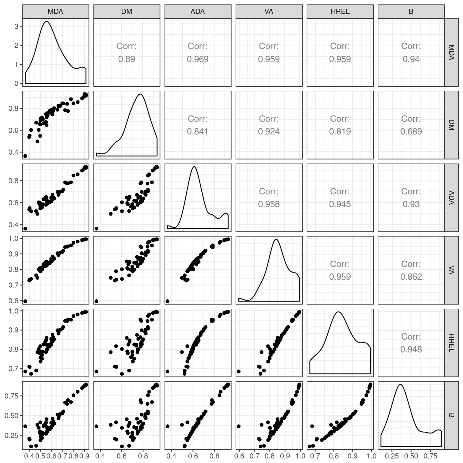
Then we can examine how these various indices are correlated. As this plot shows, all six indices are highly correlated in this example, even though the correlation between the DM and B indice is not so strong.

library(ggplot2)
library(GGally)
library(dplyr)
library(tidyr)

wilcox1973 %>%
  ggpairs(5:10) +
  theme_bw()

Scatterplots, kernel density and correlation between all six indices.

Bibliography

Kaiser, Henry F. ‘A Measure of the Population Quality of Legislative Apportionment.’ The American Political Science Review 62, no. 1 (March 1968): 208.

Senders, Virginia L. Measurement and Statistics. New York: Oxford University Press, 1958.

Wilcox, Allen R. ‘Indices of Qualitative Variation and Political Measurement.’ The Western Political Quarterly 26, no. 2 (1 June 1973): 325–43.